Demo Data Examples
This page maps the current Heliokit CLI to the sample data used by the desktop
demo workflows. Set $DEMO_DATA to the directory where those sample files are
available.
Install the host and the components used below:
python -m pip install heliokit `
  heliokit-data-cdf heliokit-data-plt heliokit-data-vti `
  heliokit-data-h5 heliokit-filter-data-calculator `
  heliokit-filter-format-convert heliokit-filter-meshtovtk-scs `
  heliokit-filter-scattertovtk heliokit-viz2d-xy-line `
  heliokit-viz2d-histogram heliokit-viz2d-histogram2d `
  heliokit-viz3d-volume heliokit-viz3d-slice `
  heliokit-viz3d-iso-surface heliokit-viz3d-wireframe
Then activate short component commands in the current terminal:
$DEMO_DATA = "D:\data\heliokit-demo-data"
$OUT = "D:\data\heliokit-demo-output"
New-Item -ItemType Directory -Force $OUT | Out-Null
heliokit activate --no-prompt | Invoke-Expression
After activation, component names can be used as short commands, such as
histogram2d or meshtovtk_scs.
Data inspection
Inspect the PSP CDF file used by the desktop XY-LINE and HISTOGRAM demos:
heliokit data read cdf "$DEMO_DATA\1D\psp_fld_l2_mag_rtn_2020010300_v02.cdf"
Inspect the PLT file used by the desktop HISTOGRAM2D demo:
heliokit data read plt "$DEMO_DATA\2D\CMF_ME.plt"
Inspect the VTI file used by VTK visualization demos:
heliokit data read vti "$DEMO_DATA\VTK\uniform_004.vti"
2D visualization
The desktop XY-LINE.swimc demo selects components from
psp_fld_l2_mag_RTN. The current CLI accepts whole dataset names rather than
component-index selectors, so the runnable examples below use the CMF PLT data
also present in the demo set.
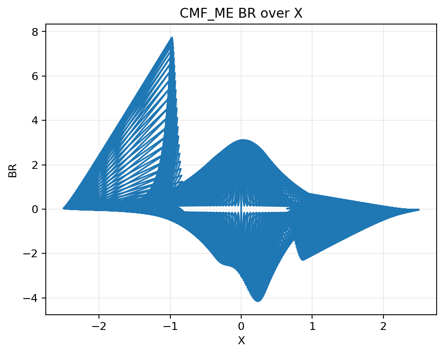
xy_line `
  --input "$DEMO_DATA\2D\CMF_ME.plt" `
  --x X `
  --y BR `
  --save "$OUT\xy_line.png" `
  --no-show
Example output:
Create a histogram from a CMF PLT variable:
histogram `
  --input "$DEMO_DATA\2D\CMF_ME.plt" `
  --array BR `
  --bins 10 `
  --save "$OUT\histogram.png" `
  --no-show
Create a 2D histogram from the CMF PLT variables used by the desktop demo:
histogram2d `
  --input "$DEMO_DATA\2D\CMF_ME.plt" `
  --x BR `
  --y BF `
  --bins 72 `
  --save "$OUT\histogram2d.png" `
  --no-show
3D VTK visualization
Render a volume screenshot from the VTI demo file:
volume `
  --input "$DEMO_DATA\VTK\uniform_004.vti" `
  --array density `
  --save "$OUT\volume.png" `
  --no-show
Render a middle-Z slice:
slice `
  --input "$DEMO_DATA\VTK\uniform_004.vti" `
  --array density `
  --axis z `
  --save "$OUT\slice.png" `
  --no-show
Render an iso-surface:
iso_surface `
  --input "$DEMO_DATA\VTK\uniform_004.vti" `
  --array density `
  --save "$OUT\iso_surface.png" `
  --no-show
Render a wireframe:
wireframe `
  --input "$DEMO_DATA\VTK\uniform_004.vti" `
  --array density `
  --save "$OUT\wireframe.png" `
  --no-show
Filters and conversion
Calculate a derived CMF magnitude from PLT variables:
data_calculator `
  --expression "sqrt(BR**2 + BF**2)" `
  --var BR="$DEMO_DATA\2D\CMF_ME.plt::BR" `
  --var BF="$DEMO_DATA\2D\CMF_ME.plt::BF" `
  --name br_bf_magnitude `
  --output "$OUT\cmf_br_bf_magnitude.h5"
Convert a spherical mesh H5 file to VTI. Radius bounds and active scalar default from the loaded data, matching the CLI default-parameter behavior.
meshtovtk_scs `
  --rad "$DEMO_DATA\3D\coronal.h5::R" `
  --theta "$DEMO_DATA\3D\coronal.h5::THETA" `
  --phi "$DEMO_DATA\3D\coronal.h5::PHI" `
  --scalar value="$DEMO_DATA\3D\coronal.h5::VALUE" `
  --size 64 `
  --output "$OUT\coronal_value.vti"
Convert scattered CMF PLT data to a sampled VTI:
scattertovtk `
  --x "$DEMO_DATA\2D\CMF_ME.plt::X" `
  --y "$DEMO_DATA\2D\CMF_ME.plt::Z" `
  --z "$DEMO_DATA\2D\CMF_ME.plt::FS" `
  --scalar BR="$DEMO_DATA\2D\CMF_ME.plt::BR" `
  --size 64 `
  --output "$OUT\cmf_scatter.vti"
Convert the CMF PLT file to HDF5:
format_convert `
  --input "$DEMO_DATA\2D\CMF_ME.plt" `
  --output "$OUT\CMF_ME.h5"
Current CLI coverage
The desktop demo states for PB, PB_FNRGF, QFactor, Twist, CMF, and several business-specific 2D tools are present in the sample state files, but their current CLI components still use placeholder adapters. They are not shown as runnable CLI examples until those runners are implemented.